Batch Normalization for faster convergence

Neural Network

Batch Normalization is not a new technique recently discovered. It was described back in 1998 by Yan LeCun, et al in the whitepaper Efficient Backdrop. But I am the kind of person that prefers visual and straighforward examples that show how the theory applies in real life. It makes things easier to remember, don't you think?

The paper explains that when the input values for the hidden layer are normalized, have close to zero average and about the same covariance, it finds the local minimum faster. This will help us stop the training process earlier by avoiding extra epochs with a proper early-stopping implementation.

For this example I am going to use a dataset that contains customer's information from a bank. The idea is to predict if the customer will leave or not the bank. Some of the independent variables we have are age, salary, if the customer is active or has a credit card and so on. In total, 8000 different fictional customers and 11 independent variables. Therefore, the score is the accuracy of our model to predict what the customer will do.

Deep Neural Network

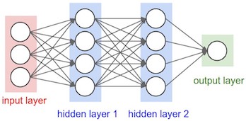
The base deep neural network will be like this:

Input layer: 11 neurons (independent variables in the dataset).
Hidden layer: 64 neurons and ReLU activation.
Hidden layer: 32 neurons and ReLU activation.
Hidden layer: 16 neurons and ReLU actication.
Output layer: 1 neuron and Sigmoid activation (probabilistic).
Backpropagation: Stochastic Gradient Descent and 0.1 learning rate.
Loss Function: Binary Cross Entropy.

For those who prefer code, here are the Keras layers:

classifier = Sequential()
classifier.add(Dense(units = 64, kernel_initializer = 'uniform', input_dim = 11))
classifier.add(Activation('relu'))
classifier.add(Dense(units = 32, kernel_initializer = 'uniform'))
classifier.add(Activation('relu'))
classifier.add(Dense(units = 16, kernel_initializer = 'uniform'))
classifier.add(Activation('relu'))
classifier.add(Dense(units = 1, kernel_initializer = 'uniform',activation = 'sigmoid'))
sgd = optimizers.SGD(lr=0.1)
classifier.compile(optimizer = sgd, loss = 'binary_crossentropy', metrics = ['accuracy'])

Train without Normalization

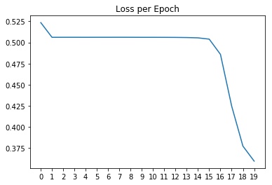
After training the Neural Network for 20 epochs the final accuracy on test set is 86,1%. Let's see how the loss changed over time on each epoch.

Loss of first NN

The graph shows how it needed up to 15 epochs to start really reducing the loss. Let's add normalization.

Train with Normalization

Normalization will be just a new layer that will be between the linear and non-linear layers in the network. That way it will normalize the input to activation functions. Again, in code:

classifier = Sequential()
classifier.add(Dense(units = 64, kernel_initializer = 'uniform', input_dim = 11))
classifier.add(BatchNormalization())
classifier.add(Activation('relu'))
classifier.add(Dense(units = 32, kernel_initializer = 'uniform'))
classifier.add(BatchNormalization())
classifier.add(Activation('relu'))
classifier.add(Dense(units = 16, kernel_initializer = 'uniform'))
classifier.add(BatchNormalization())
classifier.add(Activation('relu'))
classifier.add(Dense(units = 1, kernel_initializer = 'uniform', activation = 'sigmoid'))
sgd = optimizers.SGD(lr=0.1)
classifier.compile(optimizer = sgd, loss = 'binary_crossentropy', metrics = ['accuracy'])

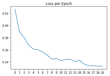
After training on 20 epocs we have an accuracy of 85,8%, 0,3% less. But remember, here the trick is not to improve the accuracy but to converge faster saving us tons of time. Let's see if that happened:

Loss of second NN

Well, looks like the graph is enough, easy to see the difference. The loss starts to lower faster since the very first epoch. We would just need to implement early-stop so the training is stopped when there are no more improvements. Saving time and $$$ if you are training on GPU cloud instances.